rNMR: Open Source Software for NMR Spectral Analysis
Ian A. Lewis and Seth C. Schommer
July 19, 2015
1 Overview
rNMR is an open source software package developed for the R statistical language environment. The rNMR package contains a collection of tools for visualizing and interpreting one and two dimensional NMR data. In contrast to most existing 2D NMR software, rNMR is specifically designed for high-throughput assignment and quantification of small molecules. As a result, rNMR supports extensive batch manipulation of plotting parameters and has numerous tools for expediting repetitive resonance assignment and quantification tasks.
The most powerful features of rNMR are built around the region of interest (ROI) concept. ROIs are user-defined chemical shift ranges that can be used to visualize and analyze hundreds of NMR signals from multiple spectra simultaneously. Unlike peak tables, ROIs are dynamic representations of the underlying NMR data. Users can actively manipulate the chemical shift ranges of ROIs while simultaneously visualizing the impact these changes will have on resonance assignments and quantification of signals.
rNMR is built on a "what you see is what you get" philosophy. Peak picking thresholds are based on the visible contour settings, ROI-based quantitative summaries are extracted from data displayed to the user, and all of the plotting and quantitative algorithms interact directly with the underlying frequency domain NMR data. This approach ensures that assignments and quantitative procedures directly reflect the NMR data visible to the users. Furthermore, this approach allows users to manipulate rNMR's quantitative algorithms by changing the graphical display settings.
Users can interact with rNMR in two major ways: via point and click graphical user interfaces (GUIs), or by entering commands directly in the R console. This flexible implementation strategy simplifies the learning process for new rNMR users while allowing more experienced R users the freedom to manipulate more advanced rNMR features. In addition, all of the underlying rNMR objects (e.g. peak tables, ROI tables, graphics settings, and raw NMR data) are accessible to users. This allows experienced R users to customize the program for more specialized applications.
This guide is intended as a brief overview of the rNMR functions, more extensive documentation can be found in the rNMR Help menu. New rNMR users are encouraged to explore the various rNMR menus, GUIs, and help pages.
2 Using R
The rNMR package runs in the R statistical computing environment. R is open-source software that is freely available from www.r-project.org. Versions of R are available for Windows, Macintosh, and Linux/Unix operating systems and rNMR can be used on any of these platforms. Under Unix/Linux operating systems, R is run from the terminal, whereas Windows and Macintosh users typically interact with R's graphical user interface (R GUI for windows, R.app for Macintosh). The default prompt in R is the ">" symbol. In this document, the ">" symbol precedes R code that can be pasted directly into R at the prompt (this is referred to as the R console). Commands in R are issued by typing the command name followed by parentheses. Arguments can be passed inside the parentheses, separated by commas, as shown below.
> sum(4, 6)
[1] 10
Help documentation for both R and rNMR functions, can be accessed by entering the command name preceded by a question mark.
> ?sum
rNMR does not require users to have an extensive understanding of R. However, R is a powerful platform for computing and graphics that is supported by an extensive library of community-developed software packages. People who are interested in customizing rNMR will find that our package, and the R environment, are well suited to add-on software development. We encourage users to explore the extensive library of packages and documentation available from www.r-project.org.
3 Installation
The rNMR package requires R version 2.10 or higher. R can be downloaded free of charge from www.r-project.org. After R has been installed, the rNMR package can be downloaded from http://rNMR.nmrfam.wisc.edu. Platform-specific instructions for installing the rNMR package are given below.
3.1 Windows
- Install R (2.10 or higher).
- Download rNMR for Windows.
- Run the rNMR installation program.
If the installation program provided in the link above does not run successfully, rNMR can also be installed using the package source.
3.2 Linux
- Install R (2.10 or higher).
- Download rNMR for Linux.
- You must change the the file permissions for the setup file before attempting to open it. You can do this by right-clicking on the file, selecting properties, and checking the execute option in the permissions tab or by typing "chmod +x" and then the filename in the terminal.
- Run the rNMR installation program.
rNMR is supported for the following Linux distributions:
- Ubuntu 8.04 (Hardy Heron) and up
- Fedora 11 (Leonidas) and up
- Redhat Enterprise Linux 4 (Nahant) and up
rNMR may run on other distributions but we can not gaurantee its performance.
If the installation program provided in the link above does not run successfully, rNMR can also be installed using the package source.
3.2 Mac OS X
- Install R (2.10 or higher)
- Download rNMR for Mac OS X.
- Run the rNMR installation program.
rNMR requires the use of a two-button mouse (CTRL+'click' is not sufficient). On most systems, the single button mouse can be configured to operate with a second button, check your systm settings. Also, rNMR is only compatible with versions of Mac OS X that come with X11 preinstalled (version 10.5 and higher). rNMR may run on older versions if X11 is installed separately, but we can not gaurantee its performance.
If the installation program provided in the link above does not run successfully, rNMR can also be installed using the package source.
4 Using rNMR
To load the rNMR package, open R and type:
> library(rNMR)
After the package has been loaded, an rNMR-specific menu bar will appear. In windows, rNMR menus are added directly to the R GUI whereas other platforms have a separate floating menu bar for rNMR. All rNMR functions can be accessed using these menus or by typing commands directly into the R console. A full list of rNMR commands can be found under the "List functions" option of the rNMR Help menu. In addition to the main rNMR menus, Windows users can right-click on any of the plot windows to view additional commands relevant to the current plot.
Many rNMR functions (including zooming and peak picking functions) require that the user interact with one of rNMR's plot windows. Calling one of these functions causes a message to be displayed detailing the required user input to execute the function. This message is displayed in the R console as well as the plot window requiring user interaction. To halt the execution of one of these functions, Windows users should right-click in the appropriate plot window and select "Stop". Linux and Macintosh users need only right-click in the plot window. Help pages for individual functions may accessed using the standard R help format, "?command", or through rNMR's Help menu. The layout for a typical rNMR session is displayed in Figure 1.
 Figure 1.
 Typical layout for the Windows version of rNMR.
5 Converting files
rNMR is compatible with UCSF (the default format for Sparky) format spectra only. Files may be converted using rNMR's file conversion function cf().
5.1 Requirements for rNMR's file converter
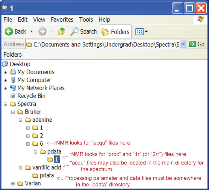
rNMR's file converter assumes a certain file structure for input directories which must be adhered to for file conversions to be successful. Bruker format spectra must contain processed data files in a folder named "pdata" (Figure 2). Processed data files must be titled "1r" (1D spectra) or "2rr" (2D spectra). This folder must also contain the processing parameter files, "procs" and "proc2s" (for 2D spectra). Acquisition parameter files, '"acqus" and "acqu2s" (for 2D spectra), must be in a directory above the "pdata" folder. These files/folders may be nested within other folders, so long as a "pdata" folder exists somewhere in the spectrum's directory.
 Figure 2.
 Bruker file structure.
NMRPipe format spectra should be individual files containing the NMRPipe format header for the spectrum followed by the processed data. These files should have a ".ft2" or ".dat" extension.
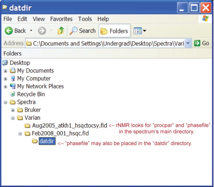
Varian format spectra must contain a processed data file ("phasefile") as well as a processing parameters file ("procpar"). The processed data must be in the directory for the spectrum or in a folder named "datdir" (Figure 3). When a spectrum is saved in Vnmr, the processed data file is not written to the same location as the saved spectrum. Instead, "phasefile" is saved to Vnmr's default experimental directory (e.g. "~/vnmrsys/exp#/datdir/phasefile"). Spectra may be converted from the "vnmrsys" directory or from the directory where the spectrum was saved, as long as the "phasefile" and "procpar" files are present. These files can be copied automatically for multiple spectra using the Vnmr macro provided at the rNMR website.
 Figure 3.
 Varian file structure.
The "phasefile" and "procpar" files can also be copied manually from the "vnmrsys" directory to the saved directory for the spectrum if the spectrum is processed correctly. To ensure proper conversion in rNMR, Varian spectra must be processed using the following commands:
- 1D spectra: fn=np*2 ft f full vsadj dc ds flush
- Arrayed 1D spectra: fn=np*2 ft f full vsadj dc dssh flush
- 2D spectra: trace='f1' wft2da f full dconi flush
These commands can be altered using the following guidelines:
- The "ft" and "wft2da" commands can be substituted with equivalent Fourier transform commands.
- Alterations to the processing parameters (e.g. zero filling, window functions, phasing) must precede the Fourier transform command.
- For 2D spectra, "trace" must be set to "f1" directly before the data is transformed.
- All commands listed above that follow the Fourier transform command are required.
- For arrayed 1D experiments, the "dssh" command is necessary to display the full array.
ASCII (plain text) spectra may be formatted in two ways. Files for one-dimensional spectra must include two columns, the first containing the chemical shift at each point in the spectrum and the second containing the intensity at each point in the spectrum. Any lines within a file that contain non-numeric values will be ignored during conversion. Two-dimensional spectra may be formatted in a similar matter, the first column containing direct chemical shifts, the second containing indirect chemical shifts, and the third containing intensities. Shifts need not be ordered under this format, as long as values in each row correspond to each other. An example is shown below.
| 1.762917332 |
23.87554312 |
-696158.872 |
| 1.762917332 |
23.91490676 |
-440679.422 |
| 1.762917332 |
23.95427039 |
-203887.875 |
| 1.762917332 |
23.99363402 |
-107499.813 |
Two-dimensional spectra may also be formatted into a matrix of intensities. Each value in the matrix must be separated by tabs or whitespace. The first row of the matrix must contain the chemical shifts in the direct dimension, in ascending order from left to right. The first column of the matrix must contain the chemical shifts in the indirect dimension, in ascending order from top to bottom. The first value in the matrix (the top, left corner) will be ignored. This format allows for quicker conversion and smaller file sizes.
| NA |
1.762917332 |
1.768888928 |
1.774860524 |
| 23.87554312 |
-696158.872 |
-132294.941 |
-824104.875 |
| 23.87554312 |
-696158.875 |
-824104.875 |
522845.753 |
| 23.91490676 |
-240679.421 |
-318409.656 |
171219.656 |
| 23.95427039 |
303887.875 |
148324.937 |
261825.687 |
Both formats require that values be written in plain text and must be separated by tabs or white space. Files must contain data for every point in the spectrum and should not be thresholded or compressed.
5.2 Using rNMR's file converter
Processed data files in Bruker, Varian, or NMRPipe format may be converted by selecting "Convert" from the File menu or by typing the following command in the R console:
> cf()

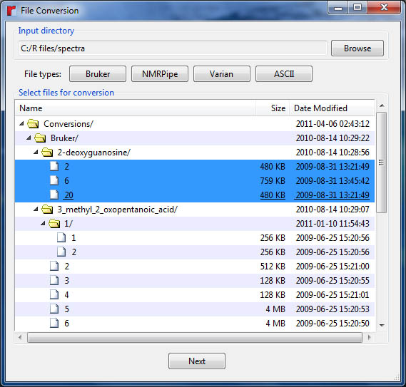
Before selecting files for conversion, the input directory must be set using the "Browse" button. This directory should contain folders for the spectra being converted or the folder for the spectrum itself. The "Bruker", "Varian", and "NMRPipe" buttons are used to find and display the appropriate files contained within the input directory. These files will be displayed in the file list box. Select the files for conversion and press the "Next" button to bring up the format-specific conversion dialog.
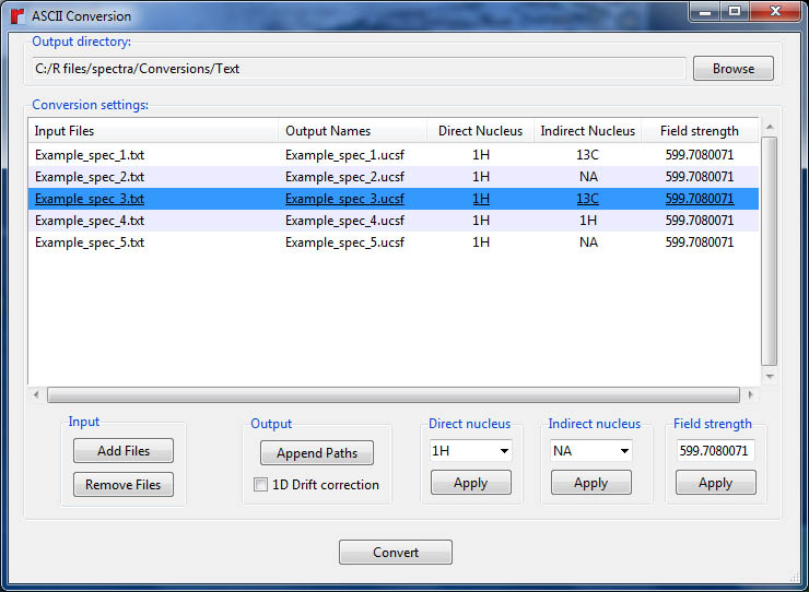
For Bruker and NMRPipe files, the "Next" button will bring up a dialog containing the selected spectra as well as the corresponding output names for the newly converted files. Click within the "Output Names" column to modify these entries. Pressing the "Append Paths" button will append the file path (relative to the original input directory) to the output name for a selected file. Checking the "1D Drift correction" box will correct DC offset problems and set the median noise level to zero for all one-dimensional spectra being converted. Once the conversion parameters have been set, press the "Convert" button to convert the displayed files to UCSF format.

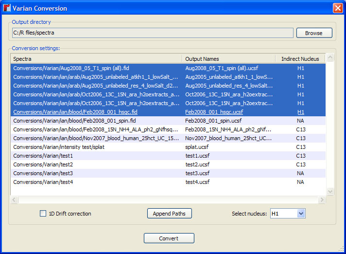
After selecting Varian files for conversion, the "Next" button will bring up a nucleus selection dialog. By default, the conversion function selects the indirect nucleus using the "dn" parameter from the spectrum's "procpar" file. If this value is incorrect, select the appropriate file along with the correct nucleus from the drop-down menus in the "Indirect Nucleus" column. Multiple entries may be modified using the nucleus selection menu at the bottom. This step is only necessary for 2D spectra. Note that rNMR's converter does support Varian arrayed 1D spectra, however, each dataset in the array will be saved to a separate file, named and numbered automatically by the converter.

5.3 Using rNMR's ASCII converter
Processed spectra in ASCII (plain text) format may be converted by pressing the "ASCII" button in the conversion dialog, or by typing the following command in the R console:
> ca()

To convert files, designate an output directory and select the files you wish to convert using the "Add Files" button. Output names may be modified by clicking within the "Output Names" column. Pressing the "Append Paths" button will append the file path to the output name for a selected file. Checking the "1D Drift correction" box will correct DC offset problems and set the median noise level to zero for all one-dimensional spectra being converted. The direct and indirect (if applicable) nuclei for each spectrum must be provided before conversion. The field strength each spectrum was collected under may also be provided, but this is optional (see help page for the ca() function for more information on this). Click anywhere within the table to edit a single entry. Multiple entries may be edited simultaneously using the options at the bottom of the GUI. Once the conversion parameters have been set, press the "Convert" button to convert the displayed files to UCSF format.
6 Viewing NMR Spectra
rNMR accepts UCSF (the default for format Sparky) format spectra only. Files in Bruker, NMRPipe, Varian, or plain text format may be converted using the cf() function detailed above.
6.1 Opening spectra
To open a spectra in rNMR, select "Open/Close Files" from the File menu or through the R console using the following command:
> fs()

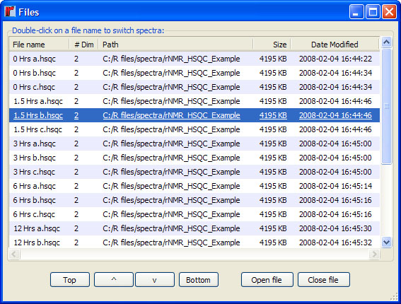
If multiple files have been opened, only the most recently opened spectrum will appear in the main plot window (Figure 4). To switch to another spectrum, double-click on a file name within the GUI. Files may be sorted using the options at the bottom of the GUI or by clicking on one of the headings in the table. To close one or more files, select the desired files from the table and then press the "Close file" button.
 Figure 4.
 The main plot window showing a sample spectrum of an
Arabidopsis extract.
6.2 Zooming and scrolling
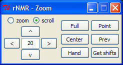
rNMR includes a wide variety of zooming and scrolling commands, all of which can be accessed through the zoom GUI by selecting "Zoom" from the View menu or by typing the following command in the R console:
> zm()

rNMR spectra may be navigated using the arrow pad provided in the zoom GUI or by using one of the five distinct zoom functions called by the buttons provided on the right side of the zoom GUI. Many of these functions are iterative and must be exited by right-clicking in the main plot window. The "Get shifts" button allows users to retrieve the chemical shifts or the chemical shift range for designated points in the main plot window.
6.3 Graphics and plotting options
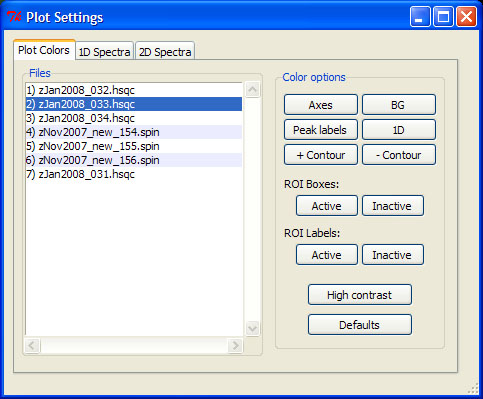
All rNMR color options and plot settings can be accessed via the Graphics menu. The co() command opens the plot colors GUI, which allows users to manipulate the color scheme used for any open spectrum. Color preferences can be applied to multiple spectra simultaneously by selecting names from the files list. Plot color options for the selected files may be configured individually using the buttons provided on the right side of the GUI. The "Axes" button changes the color of the x and y axes, "BG" changes the background color, "Peak labels" changes the label color for picked peaks, "1D" changes the color for one-dimensional spectra, and the "+ Contour" and "- Contour" buttons change the color for positive and negative contours, respectively. In contrast to the other color options, changes made to ROI colors will be applied to all open spectra. The "High contrast" button sets all color options to black or white and the "Defaults" button restores all options to their default values.
> co()

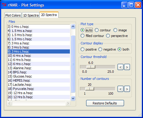
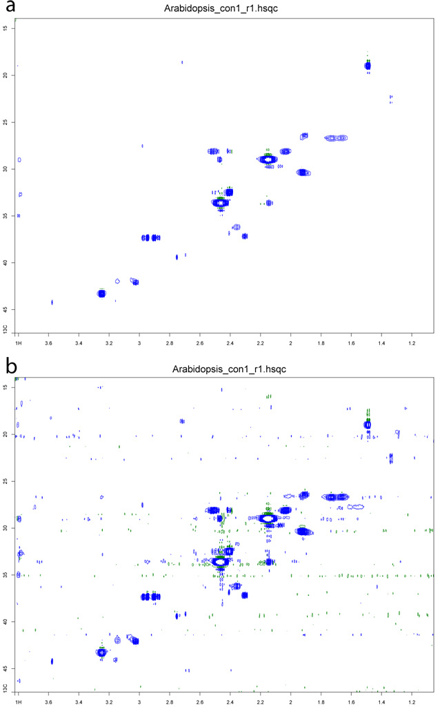
Plot features such as 2D contour level (Figure 5) and plot type can be adjusted by selecting the "Plot settings" option in the Graphics menu or through the R console using the following command:
> ct()

To apply plot settings to multiple files, select the desired spectra from the files list and choose from the available options. Double-clicking on any spectrum in the files list will switch the current spectrum to the file selected. To adjust the contour settings use the scales provided. The scales' upper limits may be adjusted using the left and right arrow buttons adjacent to each scale. This will also change the scale's resolution (increment).
In addition to altering the visual representation of the data, the plot settings GUI can be used to control peak picking and other quantitative analyses. rNMR operates under the "what you see is what you get" principle; if the negative contour display is turned off while a spectrum is peak picked, then the peak picking algorithm will ignore all of the negative signals in the spectrum (see section 8 for more on peak picking).
 Figure 5.
 A spectrum of an
Arabidopsis extract (a) before and (b) after lowering the minimum contour levels.
Two-dimensional spectra may be viewed as 3D perspective plots using the perspective GUI. The perspective GUI may be accessed through the Graphics menu, the plot settings GUI, or through the R console using the following command:
> per()

As long as the perspective GUI is open, the current spectrum will be displayed as a perspective plot, provided that the spectral window is not too large. If the current spectral width is too large for a perspective to be plotted, the plot type remains unchanged. Zooming to a smaller spectral width will redisplay the plot as a 3D perspective (Figure 6).
 Figure 6.
 A perspective plot showing a glutamine peak from an
Arabidopsis extract.
6.4 Overlaying spectra
The rNMR package includes tools for overlaying multiple spectra. We have found spectral overlays to be indispensable in assigning small molecules, particularly when it is used in conjunction with high-quality spectra from one of the small molecule standards libraries available on the web (www.bmrb.wisc.edu, http://mmcd.nmrfam.wisc.edu, and www.hmdb.ca). The rNMR overlay GUI may be accessed through the View menu or through the R console using the following command:
> ol()

To display one or more spectra on top of each other, simply select the spectra you wish to overlay from the files list and press the "Add" button. Spectra that have been added to the overlay list appear in the main plot window overlaid onto the current spectrum (Figure 7). The order in which overlaid spectra are stacked in the main spectral window is taken directly from the order of spectra appearing in the overlays list. Color options for each of the overlaid spectra can be manipulated by selecting files from the overlays list and pressing one of the three color buttons. By default, the names of overlaid spectra are displayed in the main plot window. To turn this feature off, uncheck the display option at the bottom of the GUI.
 Figure 7.
 Two standard spectra (arginine and glutamine) overlaid onto a spectrum of an
Arabidopsis extract.
6.5 1D slices and projections
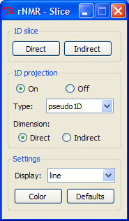
One-dimensional slices and projections may be viewed using the projections GUI. The projections GUI may accessed through the View menu or through the R console using the following command:
> pj()

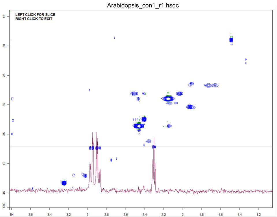
1D slices and projections may only be viewed if the current spectrum is two-dimensional. The slice buttons display a one-dimensional slice of 2D spectral data along the desired dimension (Figure 8). The location of the slice is defined by pressing one of the slice buttons followed by clicking on a point within the main plot window. This is an iterative function that can only be exited by right-clicking in the main plot window.
 Figure 8.
 The main plot window displaying a 1D slice from a spectrum of an
Arabidopsis extract.
1D projections may be displayed by turning the projection display on and selecting from the options provided in the GUI. Unlike slices, projections are one-dimensional representations of two-dimensional data. The "Type" option determines what function is applied to the 2D data in order to display it in a single dimension. For more information on projections, see the rNMR help page on 1D slices and projections by typing "?pj" in the R console.
7 Chemical shift referencing
The rNMR package includes a chemical shift referencing feature that allows multiple spectra to be referenced simultaneously. rNMR's shift referencing GUI can be accessed through the Tools menu or in the R console by typing:
> sr()

The Shift referencing GUI allows users to reference a single spectrum or several spectra simultaneously. To set a chemical shift reference, enter a numeric value for the shift (or use the "Get shift" button to use a point in the current spectrum) and then define the reference point by pressing the "Point" or "Region" buttons. These functions require the selected spectra to have been collected under similar conditions (number of points, number of dimensions, types of nuclei, etc.). Alternatively, shifts may be incrementally adjusted using the arrows found at the bottom of the GUI. Manual shift adjustments are convenient when used in conjunction with overlaid spectra of properly referenced standards (Figure 9). The number in the middle of the arrow pad is used to manipulate the manual chemical shift adjustment increment (in ppm). The "Default" button restores the original (as collected on the spectrometer) chemical shift values for the selected spectra. Chemical shift reference changes affect both the spectral display and the peak lists associated with any of the re-referenced files. ROI tables (see section 9) are not affected by chemical shift referencing.
 Figure 9.
 A spectrum of an
Arabidopsis extract (a) before and (b) after chemical shift referencing.
8 Peak picking
rNMR's peak picking feature includes a variety of automatic and manual picking functions that may be applied to spectra individually or in batch mode. The Peak picking GUI may be accessed through the Tools menu or through the R console using the following command:
> pp()

Selected files can be picked using one of the three automatic peak pick buttons, "Full", "Region","ROI". Alternatively, peak lists may be generated by hand by pressing the "Hand" button. All of the automated peak picking functions are affected by the observed plot settings; raising the contour levels will also raise the peak picking threshold (see section 6.3 for more information on changing plot settings). For 1D spectra, the peak picking thresholds can be adjusted using the"1D threshold" option in the GUI, followed by pressing the "Apply" button. The behavior of automated peak picking functions may be further modified by adjusting the "Noise filter" setting. Detailed information on the noise filter can be found on the peak picking help page (type "?pp" in the R console).
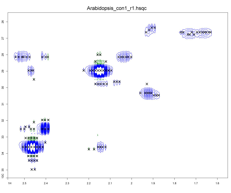
The peak list for the current spectrum may be imported or exported as tab-delimited text files using the options provided. Peak lists may also be edited within rNMR by pressing the "Edit" button. The peak list editor allows custom labels to be applied to picked peaks, which are displayed above peak markers in the main plot window. Figure 10 shows the main plot window with a peak picked spectrum displayed.
 Figure 10.
 The main plot window showing a spectrum of an
Arabidopsis extract with rNMR's peak picking markers displayed.
Several features included in the rNMR package were designed specifically for metabolomics. One such feature is the mmcd() command. The MMCD (Madison Metabolomics Consortium Database) contains an extensive collection of high quality NMR spectra and bioinformatic tools for identifying metabolites in complex solutions. The database supports multiple web-based queries and can accept peak lists uploaded from rNMR. The mmcd() command opens the MMCD homepage in the system's default web browser. Peak lists may be exported from rNMR and uploaded to the MMCD using its NMR based search in batch mode (Figure 11). Further information on the MMCD and its use is available at the MMCD homepage: http://mmcd.nmrfam.wisc.edu.
 Figure 11.
 MMCD search results from a 1H-13C rNMR peak list generated from an spectrum of an
Arabidopsis extract.
Peak lists may also be uploaded to BMRB (Biological Magnetic Resonance Data Bank) for identification. BMRB is a freely available repository for data from NMR Spectroscopy on proteins, peptides, nucleic acids, and other biomolecules. Several metabolomic data analysis tools are available at BMRB, including an NMR peaks query. The chemical shift columns from an rNMR peak list may be copied after export and pasted into BMRB's NMR Peaks Query for analysis (Figure 12). See the BMRB homepage at http://www.bmrb.wisc.edu/ for more information.
 Figure 12.
 BMRB's NMR Peaks Query tool.
9 Regions of interest
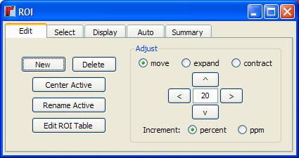
Regions of interest (ROIs) are the foundation of rNMR's most useful functions. ROIs are user-defined chemical shift ranges that can be created and edited using the ROI GUI. The ROI GUI can be accessed via the Tools menu or through the R console using the following command:
> roi()

ROIs may be generated automatically using the ra() command or by pressing the "Auto ROI" button in the ROI GUI (under the "Auto" tab). The ra() command automatically generates ROIs from visible peaks in the main plot window. New ROIs may also be created by pressing the "New" button followed by two consecutive clicks within the main plot window. This function is iterative and must be exited by right-clicking in the main plot window. Each pair of mouse clicks within the plot window indicate opposite corners of a new ROI box (Figure 13).
 Figure 13.
 ROIs corresponding to two glutamine peaks and two arginine peaks observed in a spectrum of an Arabidopsis extract.
After a set of ROIs have been created, spectral data corresponding to the ROIs may be viewed using the "Display" options in the ROI GUI. The ROI display for the currently displayed spectrum may be turned on or off by selecting the "Main window" option from the GUI. ROIs from the current spectrum may be viewed side by side using the "Subplot window" option. The "Multiple file window" option displays ROI spectral data extracted from multiple files (Figure 14). To display the maximum intensities for each ROI within this window, select the "ROI max intensities" option in the GUI.
 Figure 14.
 The multiple file window showing ROIs from eight blood samples through a 12 hour time course.
The multiple file window only displays data extracted from active ROIs. ROIs are referred to as active if they have been selected using the options provided in the "Select" tab of the ROI GUI. The majority of the available ROI functions are performed only on ROIs that are currently active. For more information on selecting ROIs refer to the help page for the rs() function.
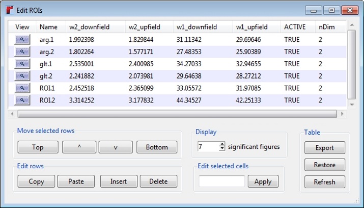
The "Edit" tab allows ROIs to be actively moved or resized to ensure that the ROIs contain only the desired peaks. Detailed information on editing ROIs can be found on the ROI help page (type "?roi" in the R console). Once created, ROIs are automatically compiled in to a table which may be imported or exported using commands in the rNMR "File" menu. The ROI table data may be edited by pressing the "Edit Table" button in the GUI, or through the R console using the command below. The ROI edit feature can be used to rename and sort ROIs or as an alternative method for moving/resizing ROIs.
> re()

Selected ROI's may be sorted using the options provided underneath the table. Cicking on a column heading in the table will sort the ROIs by the selected column. To edit an entry, click on an item in the table and enter your changes. To edit multiple entries simultaneously, select the items in the table you wish to edit, enter your changes into the text box at the bottom of the GUI, and press the "Apply" button. Rows in the table may be edited using the options provided at the bottom of the GUI. To zoom in on a specific ROI in the current spectrum, click the magnifying glass in the corresponding row in the table. Pressing the "Restore" button will undo any changes since the window was opened. The "Refresh" button updates the current table if any changes were made outside of the edit window.
Once ROIs have been created, spectral data contained within each ROI displayed in the multiple file window may be summarized using rNMR's ROI summary feature. ROI summaries may be generated using the ROI GUI or through the R console using the following command:
> rSum()

This will bring up a series of dialogs used to configure the various options available for the summary. Alternatively, summary options may be configured using the "Summary" tab in the ROI GUI (above). Summary data may include the maximum, minimum, or absolute maximum intensity from each ROI as well as the area, absolute area, or chemical shifts at the maximum intensity within each ROI. These data may be normalized using data from one or more ROIs; this is a particularly useful feature if the data includes an internal standard. Data may also be normalized using ROI summary data from one or more files, or by the constant sum of the spectral data for each file. ROI summaries are also capable of returning the signal to noise ratio for each ROI by selecting "Signal to noise" from the normalization options list.
Future versions of rNMR will include a statistics module to facilitate further analysis of ROI summary data. Currently, ROI summaries can be exported (via the export command found in the File menu) as tab-delimited files that can be read directly by spreadsheet software such as Microsoft Excel®. Data can also be extracted from the main plot window or any of the rNMR tables for analysis within R using the ed() function (select "extract data" from the Tools menu).
10 Preferences
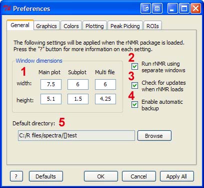
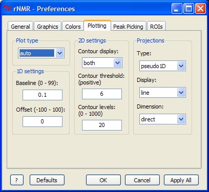
rNMR loads with a set of default preferences, such as graphics and plot settings, which can be modified by selecting "Preferences" from the Edit menu or by typing the following in the R console:
> ep()
Changes made in the preferences GUI may be saved in two ways. Pressing the "OK" button saves the updated preferences but will not apply any changes until the next time rNMR loads or a new spectrum is opened. The exception to this rule are global settings. These are settings that are applied to all spectra and plot windows, such as ROI color and auto generation settings. Modifications to these settings will be visible on the next plot refresh (or the next time the plot window is closed and reopened). Alternatively, changes can be applied immediately using the "Apply All" button. Note that this will save and apply all settings for each tab in the GUI to all open spectra. The "Defaults" button restores the default settings for the currently displayed tab (settings will not be saved until the "OK" or "Apply All" button is pressed).
10.1 General preferences

1 - Plot window dimensions in inches. Changes will not be applied until the affected window is closed and reopened (or the "Apply All" button is pressed).
2 - This option enables Rgui's SDI setting (on Windows platforms). Under the default setting (recommended), the R console and plots are placed in separate windows. Changes to this setting will be applied when R is restarted.
3 - When enabled, rNMR will check for updates when the package loads. If updates are available, rNMR will be updated automatically.
4 - When enabled, rNMR will save a backup copy of the current workspace at regular intervals. Note that this may cause rNMR to run slowly if the workspace contains a large amount of data. Use rb() to restore the most recently saved backup.
5 - The default working directory when rNMR loads.
10.2 Graphics preferences

1 - Specifies the margin size (in lines) for the various plot windows. Changes are not applied until the plot window is closed and reopened (or the "Apply All" button is pressed).
2 - Displays gridlines along the x and y axes in the main plot window.
3 - Text magnification for the various plot windows (R's "cex" graphical parameter).
10.3 Color preferences

1 - The default colors for ROIs.
2 - The default plot colors.
3 - This option sets the background color to white and the rest of the colors to black, with the exception of the active ROIs, which will remain red.
4 - Restores the default settings for the color options only.
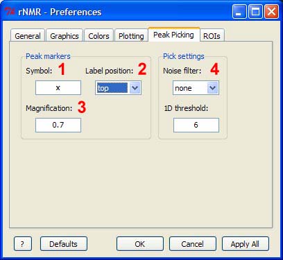
10.5 Peak picking preferences

1 - The symbol used for picked peaks (R's "pch" graphical parameter). Any ASCII (standard characters found on a keyboard) may be used as well as various numeric values which are associated with specific symbols in R. Type "?par" in the R console for more information.
2 - Peak label alignment.
3 - Peak label and symbol magnification (R's "cex" graphical parameter). The value provided here will be used when the spectrum is zoomed to full and will then be scaled depending on changes to the zoom level.
4 - These settings may be found in the peak picking GUI and are discussed in detail in the peak picking section.
10.6 ROI preferences

1 - The box type for active and inactive ROIs (R's "lty" graphical parameter).
2 - The line width for active and inactive ROI boxes (R's "lwd" graphical parameter).
3 - Text magnification for active and inactive ROI labels (R's "cex" graphical parameter).
4 - ROI label alignment, relative to the ROI box.
5 - Size (in ppm) for ROIs generated automatically using ra(). If enabled, ROI boxes will have the specified fixed width and height.
6 - Padding percentage applied to ROIs generated automatically using ra(). This padding is added to the area surrounding the peaks within an ROI and is only applied if a fixed width/height is not provided.
7 - Noise filter for ROIs generated automatically using ra(). The ra() function uses rNMR's peak picking algorithm to define ROIs, which uses this filter to determine which peaks to pick. Type "?pp" in the R console for more information on this setting.

